#analogcomputer

divmondes@pod.geraspora.de

Maybe too late for Valentines day, however today I generated the attached curve with my #analogcomputer .
Differential equation is r''=omega^2*r -g*sin(omega*t+phi0), a mass in a vertically rotating tube. r and thus the display shows the position of the mass in the xy-space.

divmondes@pod.geraspora.de

#AnalogComputer

Application: A comet moves on a parabolic orbit in the gravitational field of the stationary sun. Its orbital plane coincides with the plane of the Earth's orbit, which is assumed to be circular. The perihelion distance is one third of the Earth's orbital radius RE.
How long does the comet move within the Earth's orbit?

In the end, an integral has to be solved which also can be done with an analog computer. Details are again available at:
https://permondes.de/gitweb/Analog_Engine.git

Scaling leads again to some funny units. Time is measured in 10 kilo-days, distance in Tera-meters.

In this example, also the interim values can be displayed which is quite instructive.

An issue was the fact that for the calculation of a root, the multiplier was used in a feedback configuration. This was extremely sensitive to any signal >0 which put the circuit to an irreversible overload. Only unplugging and re-plugging the inputs to the multiplier allowed a reset.

divmondes@pod.geraspora.de

#AnalogComputer

"Calculate the trajectory of a mass with charge in a static electromagnetic field."
This was an exercise during my university studies. Lots of maths to finally find the cycloidal motion of the particle based on the differential equation set x''=omega*z', z''=a*omega^2 - omega*x'.
Simulation with the analog computer gives an impression of the behaviour when parameters are changing. Also adding initial speed (which was not part of the exercise) is really easy with fun.

1st image: the cycloidal motion.
2nd with added speed in x and z direction.

Details as usual at https://permondes.de/gitweb/Analog_Engine.git

divmondes@pod.geraspora.de

Analog Computer - Scaling

Analog engines are working with values within the range [-1, +1], thus all values have to be scaled to fit into this range at any time.
I think, this is one of the biggest challenges when realizing an application.
The example about the damped harmonic oscillator was extended to include amplitude scaling as well as time scaling.
The parameter TIMEBASE was added to the scripting language.

The files can be found in my GIT repository https://permondes.de/gitweb/Analog_Engine.git

#analogcomputer #THAT #Anabrid

divmondes@pod.geraspora.de

Analog Computer

Damped harmonic oscillator

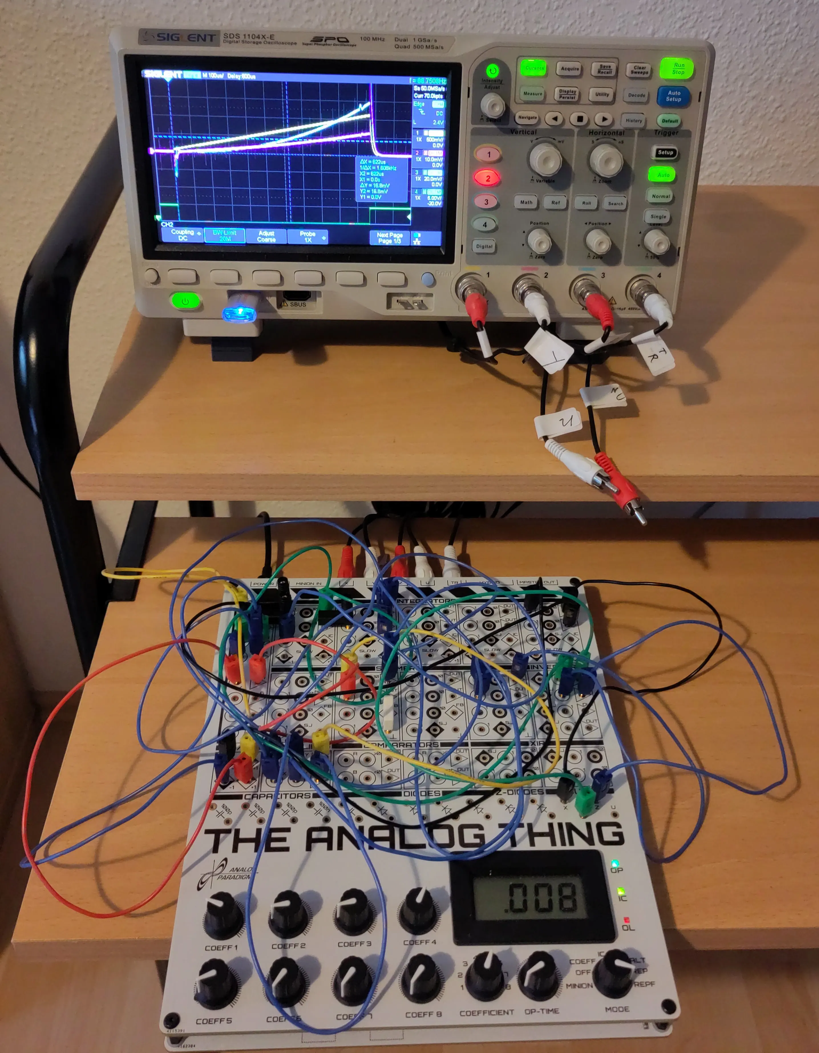
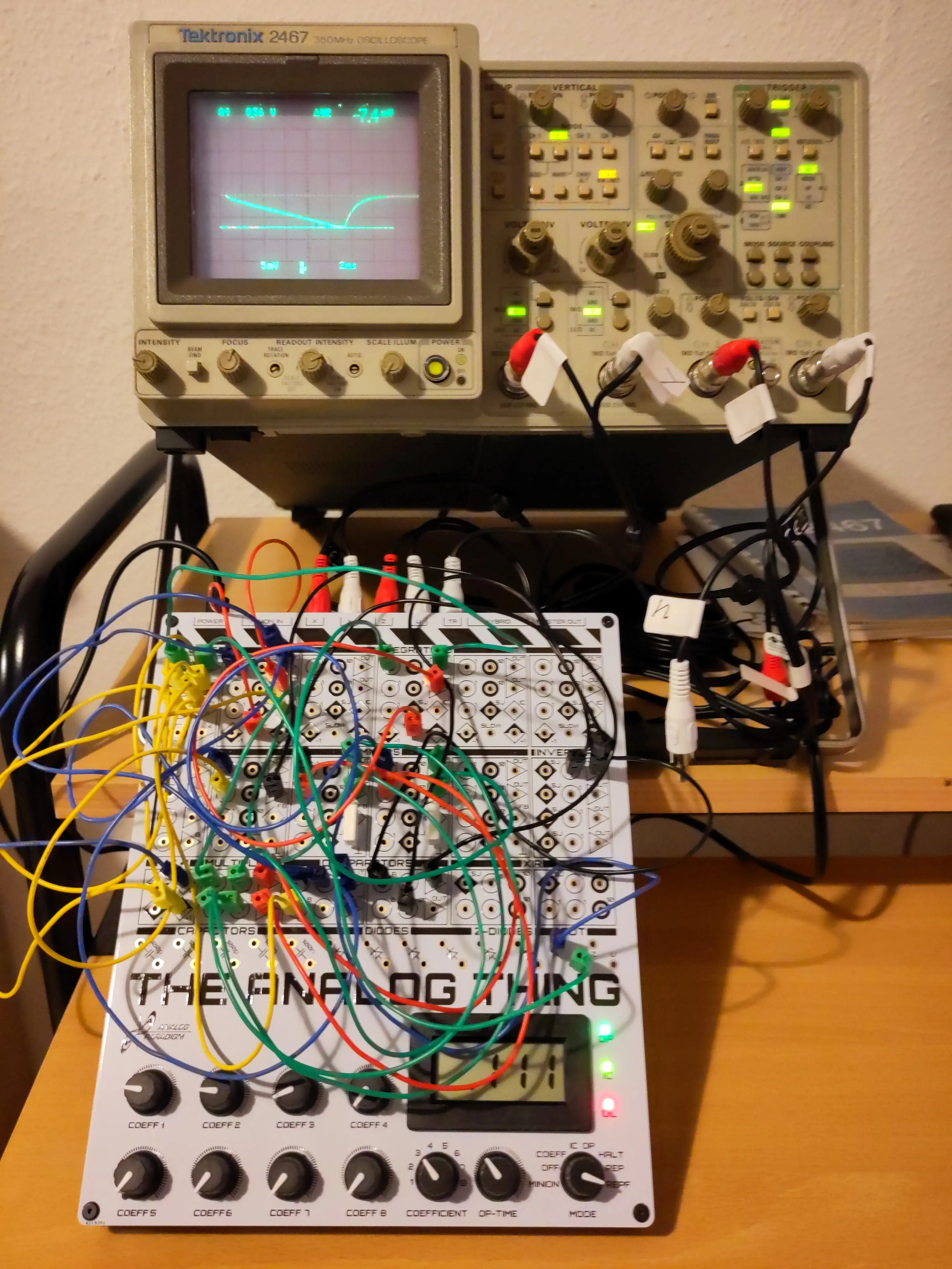
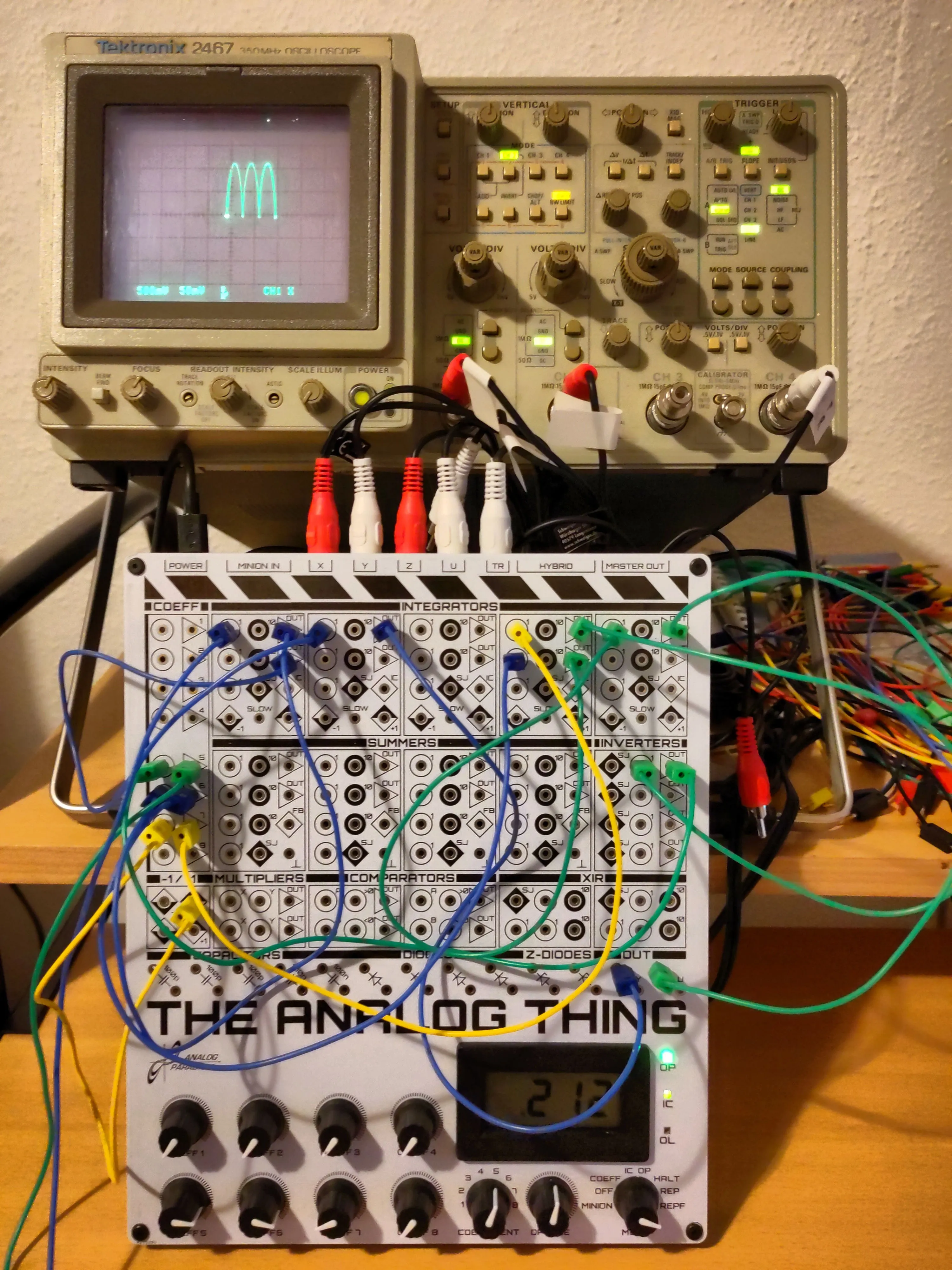
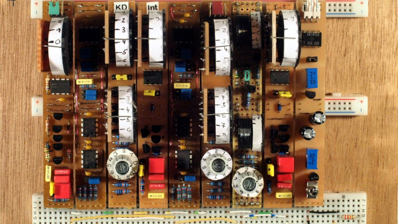
Some days ago I finally received my #analogcomputer #THAT from #Anabrid.
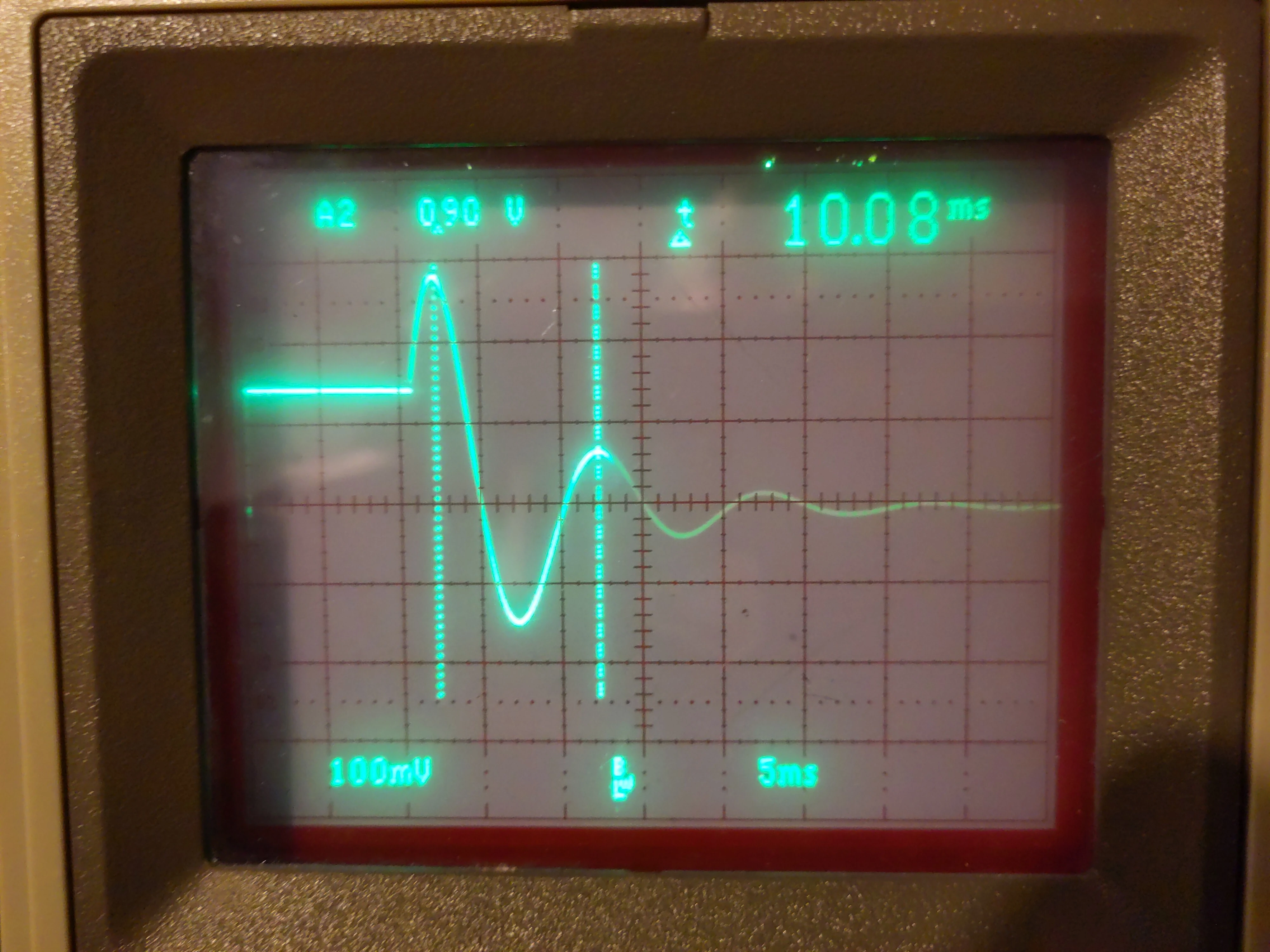
The very first trials were easy, the first real application is this damped harmonic oscillator, like a suspension of a car, a pendulum in air or a spring in air.
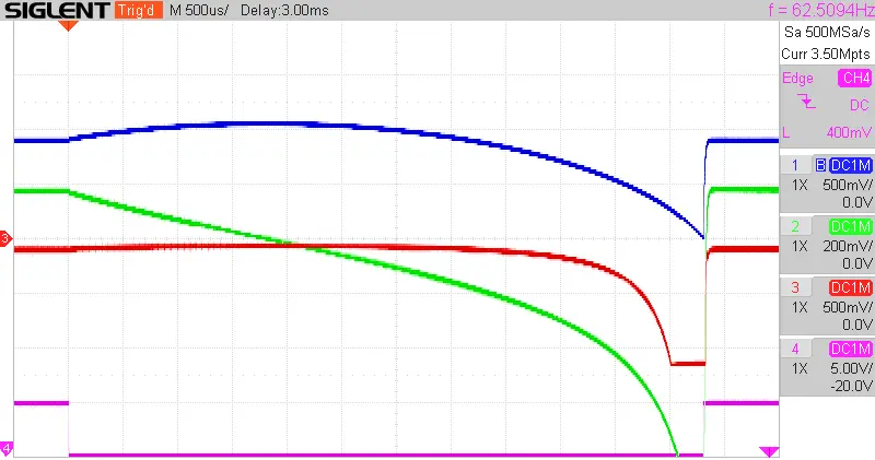
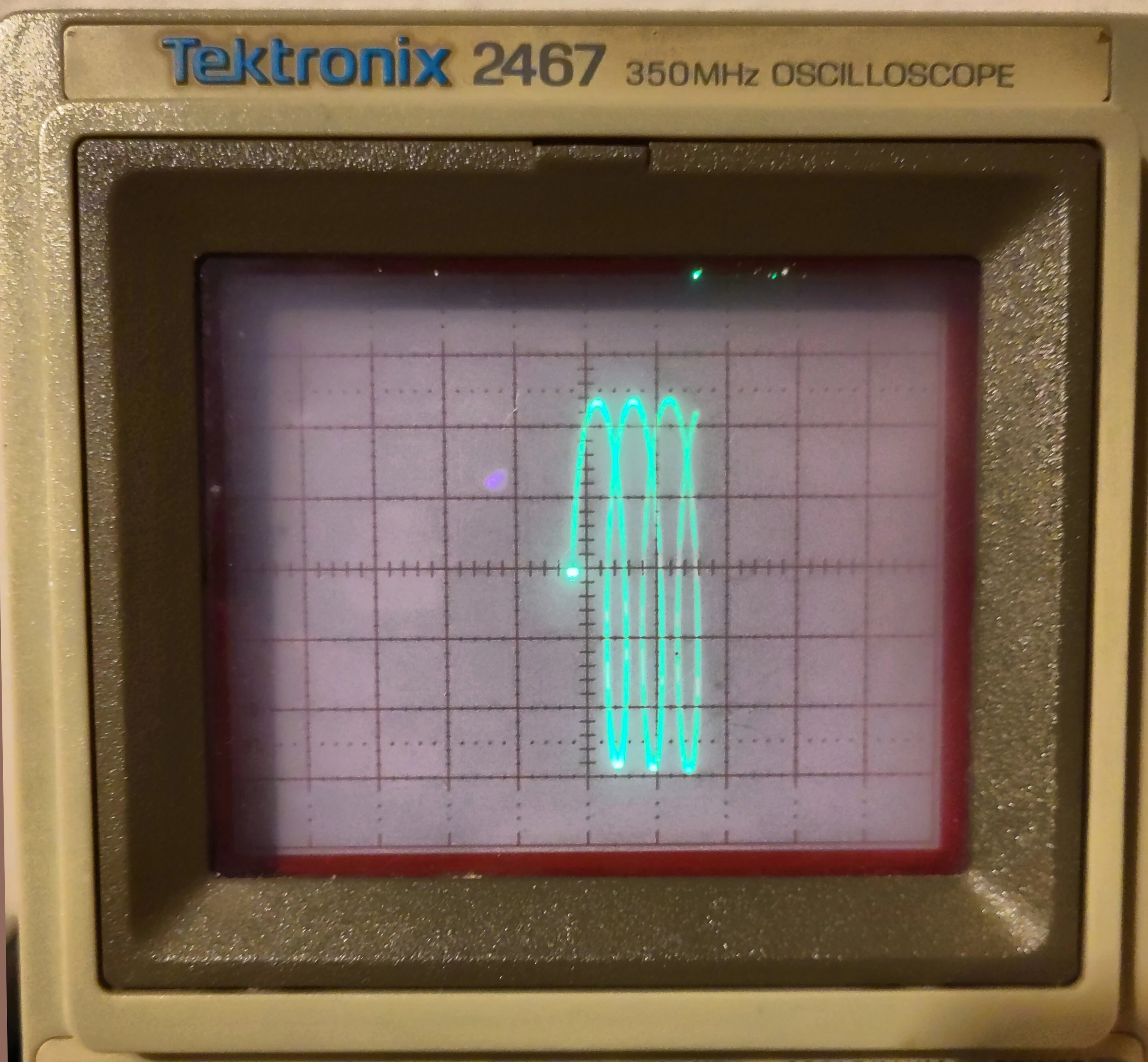
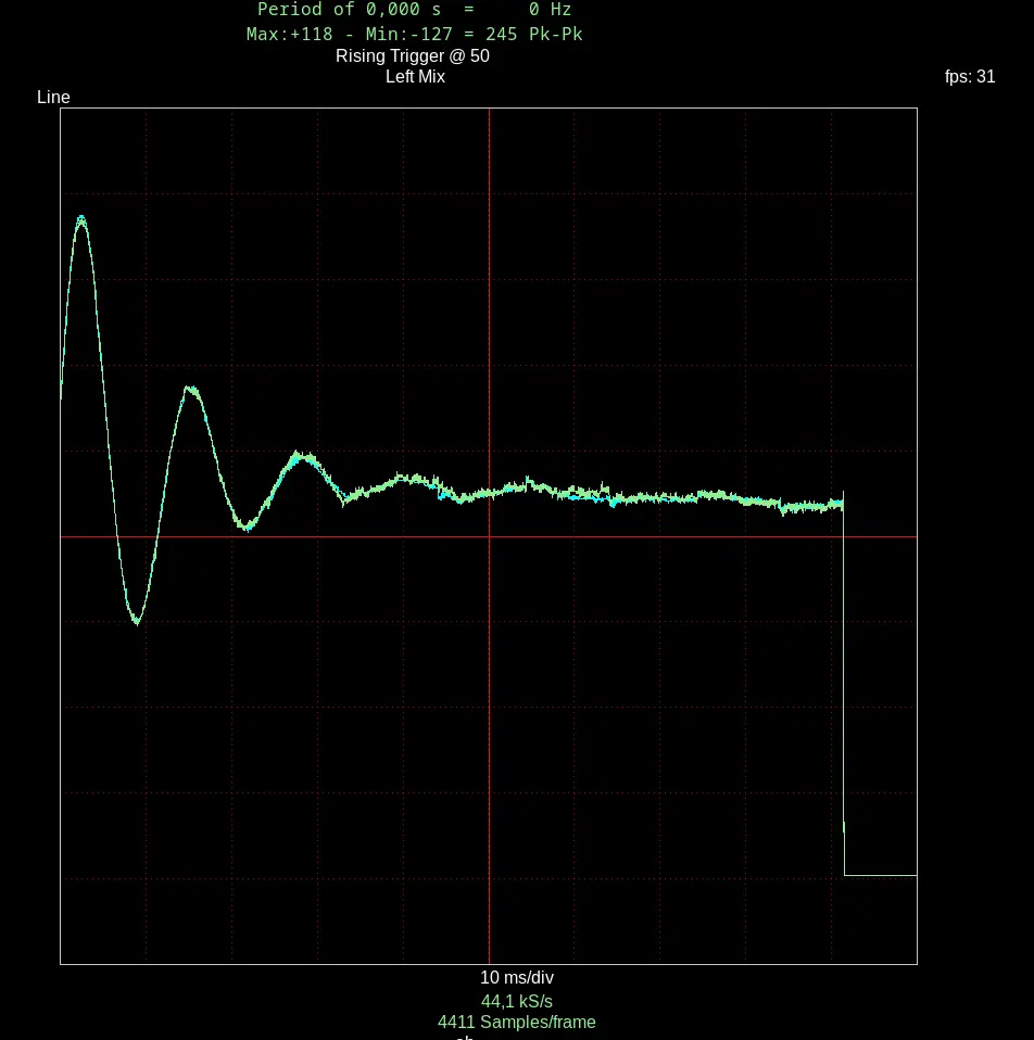
Attached is the output of such a system in a not optimized way. As can be seen, the oscillations go on for a while before being fully damped. It is easy to adjust spring constant and damping to optimize this circuit.
Further parameters are the mass (used here just to keep the amplitude in range) and the initial speed.
The circuit was realized as said above with an Anabrid-THAT, the visualization with the linux software Xoscope (I am still waiting for my physical oscilloscope).

Differential equation: my’’ + Dy’ + Sy = 0, with m the mass, D the damping with speed and S the spring constant. Rewritten to y’’=-1/m * (Dy’+Sy).
An initial condition is required; we put the deflection to y0 and the speed to y0’.

The wiring is described below. Note that I am using my own "Analog Engine Scripting Language". The syntax and further examples can be found in my git repository https://permondes.de/gitweb/Analog_Engine.git/tree

IDENTIFICATION DIVISION
PROGRAM-ID Damped_Oscillator

ENVIRONMENT DIVISION
ENGINE Anabrid-THAT
REQUIRES COEFFICIENT 5
REQUIRES INTEGRATOR 2
REQUIRES INVERTER 1
REQUIRES SUMMER 2

DATA DIVISION
OUTPUT OUT_u y
COEFFICIENT.1 -y0 # -initial position
Coefficient.2 y0s’  # initial speed
COEFFICIENT.3 S   # spring force
COEFFICIENT.4 D   # damping, linear to speed
COEFFICIENT.5 1/m # 1 / mass

PROGRAM DIVISION
# Colors being used for wiring
# - black:  y0
# - blue:   y0’
# - green:  y0’’
# - yellow: y’’, y’
# - red:    y
-1 -> COEFFICIENT.1 -> -y0 # -initial position of the mass
-1 -> Coefficient.2 -> y0s’ # y’ is scaled to be within -1..+1
+1, y0s’, y0s’ -> Summer.1 -> y0’

y’’, IC:y0’ -> INTEGRATOR.1 -> -y’
-y’,IC:-y0 -> INTEGRATOR.2 -> y
y -> COEFFICIENT.3 -> S*y # springforce times displacement
-y’ -> INVERTER.1 -> y’
y’ -> COEFFICIENT.4 -> D*y’ # damping times speed
S*y, D*y’ -> SUMMER.2 -> -(Dy’+Sy)
-(Dy’+Sy) -> COEFFICIENT.5 -> -1/m*(Dy’+Sy)=y’’

OPERATION DIVISION
MODE REPEAT
SPEED 80ms # REPF 0.800; Osci: 10 ms/div, trigger: rising at 50